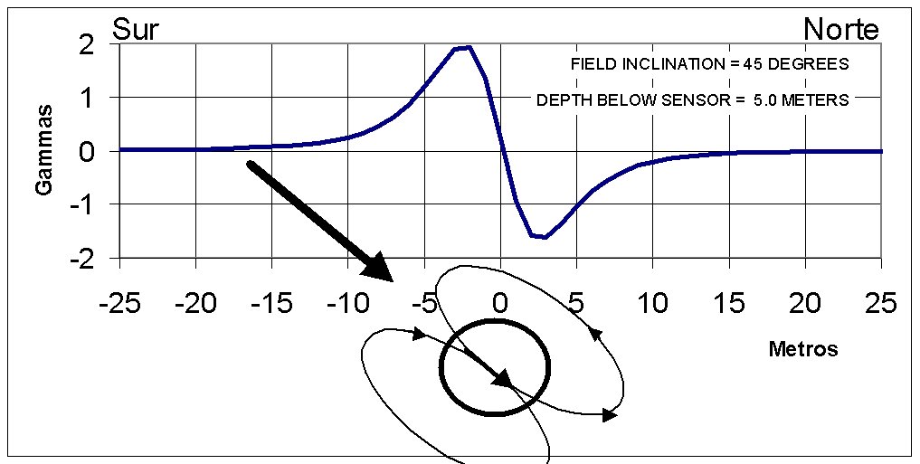
Figure 4: Shape of total field anomaly over a buried dipole.

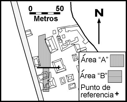
Figure 5: Areas of the Talgua site investigated with the magnetometer.

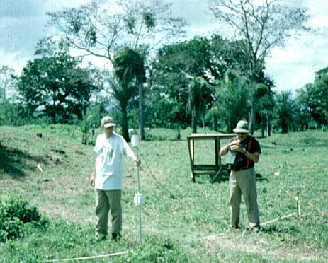
Figure 6: Geophysicists with the magnetometer at Talgua.  One carries the sensors (2, in vertical gradient configuration) in his left hand.  The second geophysicist carries the electronics unit and power supply.

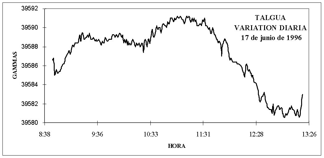
Figure 7: Example of diurnal variation, measured by the base station at Talgua, June 17, 1996.

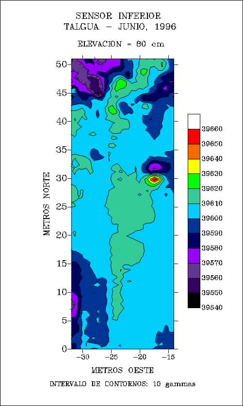
Figure 8:  Contour map showing lower sensor results, geomagnetic measurements, Area A of Talgua (see Figure 5).

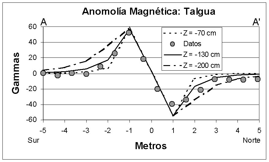Figure 9: Profile AA' from Figure 8, comparing observed anomaly with magnetic response of magnetic dipoles buried at various depths under the surface.  The Z = -70 cm curve is too narrow and the Z = -200 cm curve too broad.  The object responsible for this anomaly must lie between 70 and 200 cm deep.  A spreadsheet that calculates hypothetical anomalies can be found at http://www.geology.utoledo.edu/department/faculty/djs/MISC/SandF.htm.

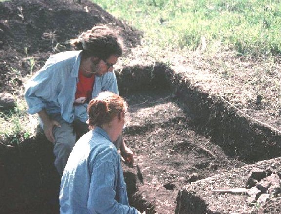Figure 10:  Archaeology students examine an ancient fire pit.   To the right are angular, fire-cracked rocks.

 
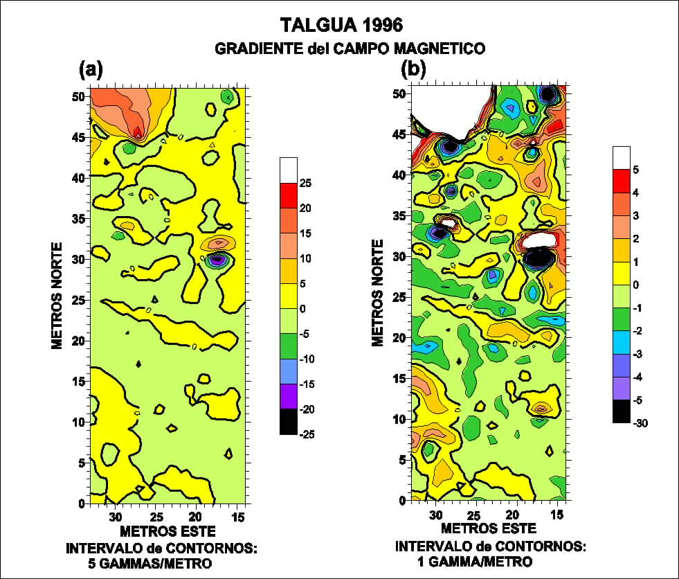
Figure 11: Gradient of the geomagnetic field, Area A (Figure 5).  Subtle anomalies become visible then the contour interval is reduced (Map b).

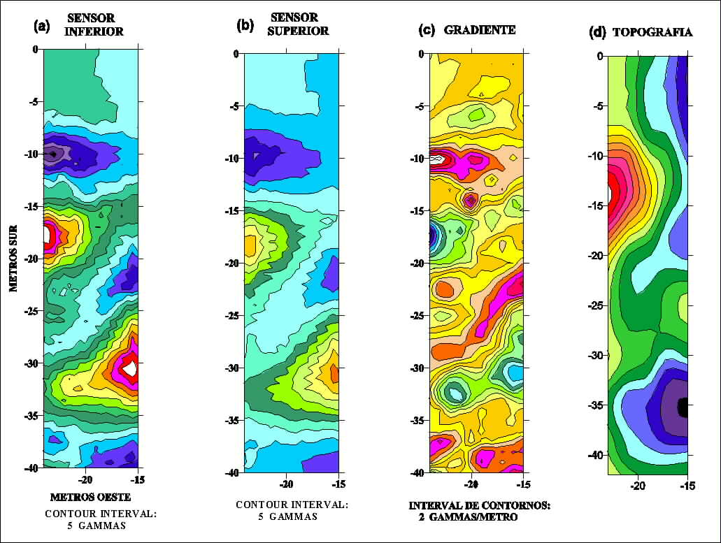
Figure 12: Geomagnetic field (12a y 12b), gradient of the geomagnetic field (12c) and topography (12d), Area B (Fig. 5).

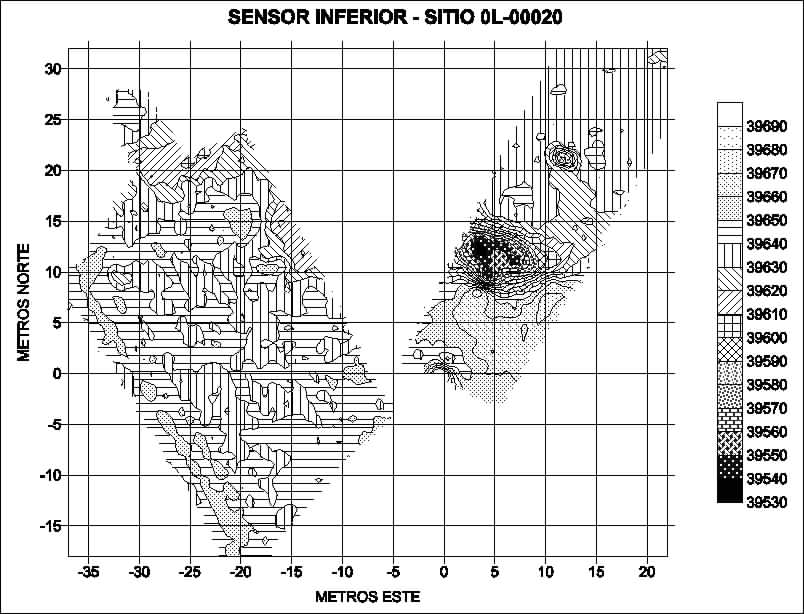Figure 13: Geomagnetic field at site 0L-00020 (Gómez, 1995).  The anomaly at (0,0) is due to the iron rod used as a reference point for the site.  The strong anomaly at (6, 12) is due to topography.

Return to Section 2 of report